libeblearn tutorial: energy-based learning in C++

By Pierre Sermanet and Yann LeCun (New York University)

The eblearn (energy-based learning) C++ library libeblearn contains machine learning algorithms which can be used for computer vision. The library has a generic and modular architecture, allowing easy prototyping and building of different algorithms (supervised or unsupervised learning) and configurations from basic modules. Those algorithms were used for a variety for applications, including robotics with the Learning Applied to Ground Robots DARPA project (LAGR).

Energy-based learning

What is the energy-based learning?
FIXME.

More resources on energy-based models:

[video-lecture] Energy-based models & Learning for Invariant Image Recognition: a 4-hour video of a tutorial on energy-based models by Yann LeCun at the Machine Learning Summer School in Chicago in 2005.
http://www.cs.nyu.edu/~yann/research/ebm/index.html: tutorials, talks, videos and publications on EBMs.
[LeCun et al 2006]: A Tutorial on Energy-Based Learning, in Bakir et al. (eds) "Predicting Structured Outputs", MIT Press 2006: a 60-page tutorial on energy-based learning, with an emphasis on structured-output models. The tutorial includes an annotated bibliography of discriminative learning, with a simple view of CRF, maximum-margin Markov nets, and graph transformer networks.

Modular Architecture and Building Blocks

Eblearn was designed to be modular so that any module can be arranged is different ways with other modules to form different layers and different machines. There are 2 main types of modules (declared in EblArch.h):

module_1_1: a module with 1 input and 1 output.
module_2_1: a module with 2 inputs and 1 output.

Each module derives from one of those two base classes and implements the fprop, bprop, bbprop and forget methods:

fprop: the forward-propagation method which propagates the input(s) through the module to the output. In the rest of this tutorial, a module will usually be described by what its fprop method does.
bprop: the backward-propagation method which propagates back the output though the module and the input(s). This method usually updates the parameters to be learned inside the module using for example derivatives, and also propagates derivatives to the input of the module so that preceding modules can also be back-propagated.
bbprop: the second-order backward-propagation method. In the case of the Lenet networks for example, this is used to compute second-order derivatives and adapt learning rates accordingly for each parameter to speed-up the learning process.
forget: initializes the weights of the modules to random, based on a forget_param_linear object.

Note that the type of inputs and outputs the modules accept are state_idx objects which are temporary buffers containing the results of a module's processing. For example, an fprop call will fill the x slot of the output state_idx, whereas a bprop call will fill the dx slot of the input state_idx (using the dx slot of the output state_idx).

Next we describe some modules and show how they are combined with other modules. We first talk about a few basic modules, which are then used to form layers that are again used to form machines. Note that all the modules that we are describing (basic modules, layers and machines) derive from module_1_1 or module_2_1 which means that you can write and combine your own modules in your own ways, which are not restricted to the way we describe here.

Basic module examples

constant addition, linear, convolution and subsampling modules

Those basic modules (found in EblBasic.h) are used in the LeNet architecture to perform the basic operations:

addc_module: this module adds a constant to each element of the input and puts the result in the output.
linear_module: this module does a linear combination of the input and its internal weights and puts the result in the output.
convolution_module_2D: convolves 2D input (dimensions 1 and 2, dimension 0 may have a size more than 1) using the internal weights as kernels and puts the result in the output.
subsampling_module_2D: subsamples 2D input (dimensions 1 and 2) and puts the result in the output.

non-linear modules

These modules (EblNonLinearity.h) perform non-linear operations:

tanh_module: applies the hyperbolic tangent function on the input and puts the result in the output.
stdsigmoid_module: applies the standard sigmoid function on the input and puts the result in the output.

Layer module examples

These layers (EblLayers.h) are built by stacking the basic modules described previously on top of each other to form more complicated operations:

nn_layer_full: a fully-connected layer which performs a linear combination of the input and the internal weights, adds a bias and applies a sigmoid. As always, the result is put in the output. This layer is build by stacking up a linear_module_replicable (see Replicability), an addc_module and a tanh_module.
nn_layer_convolution: a convolution layer which performs a 2D convolution on the input, adds a bias and applies a sigmoid, putting the result in the output. This layer is build by stacking up a convolution_module_2D_replicable, an addc_module and a tanh_module.
nn_layer_subsampling: a subsampling layer which subsamples the input, adds a bias and applies a sigmoid, putting the results in the output. This layer is build by stacking up a subsampling_module_2D_replicable, an addc_module and a tanh_module.

Machine module examples

Like the layers are built by assembling basic modules, machines (EblMachines.h) can be built by assembling layers together, for instance the following machines:

b. Overview of the architecture of the supervised_euclidean_machine, a module_2_1 (2 inputs and 1 output) that combine many module_1_1 (1 input and 1 output) modules and one module_2_1, the euclidean_module. This architecture is useful during the training phase where the bprop method is called, whereas during the testing phase only the lenet7 block will be used and only the fprop method will be called. Note that state_idx::x are temporary buffers containing outputs of fprops in between modules and state_idx::dx contain outputs of bprops.

nn_machine_cscscf: a LeNet type machine which calls in order the following layers: convolution (c), subsampling (s), convolution (c), subsampling (s), convolution (c) and finally a fully-connected layer (f). This machine is parametrized by the size of the input, the sizes of the convolution and subsampling kernels, the size of the fully connected layer output and the number of outputs.
lenet5: this machine is a nn_machine_cscscf with a particular configuration, it takes a 32x32 input, then applies 5x5 convolution kernels, 2x2 subsampling kernels, 5x5 convolutions, 2x2 subsamplings, 1x1 convolutions and full connections between a 120-dimensional input to 10 outputs. This specific network is used for the 10-digits handwriten caracters recognition (see MNIST demo).
lenet7: similarly to lenet5, this machine is a nn_machine_cscscf with a particular configuration. It takes a 96x96 input, then applies 5x5 convolution kernels, 4x4 subsampling kernels, 6x6 convolutions, 3x3 subsamplings, 6x6 convolutions and full connections between a 100-dimensional input to 5 outputs. This network was specifically designed for the NORB demo but can be an inspiration for similar object recognition tasks.
lenet7_binocular: This network is almost identical to lenet7 except that it accepts stereoscopic images as input.

a. The lenet7_binocular neural network architecture: there are 2 stereoscopic 96x96 images as input, 5x5 convolutions are performed, then 4x4 subsampling, 6x6 convolutions, 3x3 subsampling, 6x6 convolutions and full connections to the 5 outputs.

Trainable machine modules

The modules described in the previous sections need to be encapsulated in a module_2_1 with a loss function modules in order to be trained supervised. For example, to train the nn_machine_cscscf machines, we combine it with a euclidean cost module:

supervised_euclidean_machine: a module_2_1 machine containing a module_1_1 (in the NORB demo case a lenet7 machine) and a euclidean_module. Thus this machines takes an input which is propagated in the module_1_1 and a groundtruth label as second input. The output of the module_1_1 is then compared to the groundtruth using the euclidean_module which takes the squared distance between the output and the groundtruth. During the training phase, the weights are then modified based on the gradient of the error in the back-propagation process.

Module Replicability

Modules usually operate on a specific number of dimensions, for example the convolution_module_2D only accepts inputs with 3 dimensions (because it applies 2D convolution on dimensions 1 and 2, dimension 0 is used according to a connection table). Thus if extra dimensions are present (e.g. 4D or 5D) one might want to loop over the extra dimensions and call the convolution_module_2 on each 3D subsets. We call this replicability because the module is replicated over the 3rd and 4th dimensions (the output also has 2 extra dimensions).

To make a module replicable, use the DECLARE_REPLICABLE_MODULE_1_1 macro (in EblArch.h). It will automatically declare your module_1_1 as replicable and loop over extra dimensions if present. For example, here is the code to declare the convolution_module_2D as replicable:

DECLARE_REPLICABLE_MODULE_1_1(linear_module_replicable, 
                              linear_module,
                              (parameter &p, intg in, intg out),
                              (p, in, out));

where linear_module_replicable is the name of the new module, linear_module is the name of the base module, (parameter &p, intg in, intg out) is the prototype of the parameters to the constructor of the module and (p, in, out) the parameters themselves.

c. Example display of the eblearn GUI. A call to module_1_1::display_fprop will display all the internal feature maps and their corresponding description and sizes, providing that each module implemented their display method. On top are the input images, at the bottom the network outputs.

GUI display

If the QT library is present on your system, the eblearn project will automatically compile the GUI libraries corresponding to libidx and libeblearn. Thus it produces the libeblearngui library which provides display functions for the eblearn modules. For instance, it implements the display_fprop methods for each module_1_1, thus allowing to display every stage of the internal representations of the neural network by calling that method on the top-level module (See figure c).

For more details about the GUI features, refer to the GUI section in the libidx tutorial. Briefly, the libidxgui provides a global object "gui" which can open new windows (gui.new_window()), draw matrices (gui.draw_matrix()), draw text (gui << at(42, 42) << "42" << endl) and some other functionalities.

Supervised Learning

Eblearn provides supervised learning algorithms as well as semi-supervised and unsupervised ones. They can be used independently or combined, we will focus on supervised algorithms only in this section.

1. Build your dataset

What data should you provide to the network?

Creating datasets from image directories

Once you have grouped all your images in different directories for each class, call the dscompile tool to transform them into a dataset object (a matrix of images with their corresponding label). This tool will extract the label information from the file directory structure: at the source level, each directory is a class named after the directory name. Then all images found in subdirectories (regardless of their names or hierarchy) are assigned the same label and are added to the dataset.

For example with the following directory structrure, dscompile will automatically build a dataset with 2 different labels, "car" and "human" and will contain 5 images in total:

/data$ ls -R *
car:
auto.png  car01.png

human:
human1  human2

human/human1:
img01.png

human/human2:
img01.png  img02.png

dscompile will create the following files:

dset_data.mat: a ubyte matrix of size N x M x height x width , where N is the number of images and M the number of channels which can be 1 or 3 if the input images are in greyscale or color or 2 or 6 if two (stereoscopic) images are passed instead of one. Here are the possible channel configurations: G or GG, RGB or RGBRGB.
dset_labels.mat: an int matrix of size Nclasses containing labels id numbers, e.g. 0, 1, ...
dset_classes.mat: a ubyte matrix of size Nclasses x 128 containing the names of each class.

For more details, see the tools manuals of dscompile, dssplit, dsmerge, and dsdisplay.

d. Example display of the MNIST dataset after a call to LabeledDataSource::display(), which displays groundtruth (left), correct and incorrect answers (middle) and incorrect only (right).

Loading datasets into a LabeledDataSource object

2. Build your network

The eblearn neural networks are build by combining modules together as introduced at the beginning of this tutorial. Depending on your application, you may want to write your own modules or combine already existing modules in different ways. For example for simple applications (See Perceptron demo), you may want to have just one fully-connected layer in your machine. For more complex tasks, some architectures are already built-in, such as the lenet5 and lenet7 architectures. The lenet5 and lenet7 classes derive from the nn_machine_cscscf class and only specify specific sizes for the input, kernels and outputs. As described earlier, the lenet5 architecture is capable of learning handwritten caracter recognition (10 categories) while the lenet7 was used for object recognition (5 categories).

Your application will probably be different than the MNIST or NORB applications but if your goal is object recognition you want to reuse the nn_machine_cscscf class and the lenet5 or lenet7 parameters but change a few of them (See the constructors of lenet5 and lenet7 for more details). The main changes you will have to do are:

number of outputs: for MNIST this is equal to 10 and for NORB it is 5. If you attempt to build a system that can recognize 15 different categories, this value will be 15.
size of the input: this is 1x32x32 for MNIST, 1x96x96 for NORB and 2x96x96 for the binocular version of NORB. If you have multiple channels (e.g. RGB, YUV or binocular greyscale inputs), you may have to rework the connection table between the input and the first convolution layer.
connection tables: if there is no pre-configured network with the same number of input channels as you do, you have to modify the connection table with the first layer. In nn_machine_cscscf, this table is the table0 object in the constructors in EblMachines.cpp. It specifies which input channels will be convolved into which feature map. For example in lenet7, it's a full table of size 6 because the only greyscale channel is connected to all 6 features maps of the first convolution. Whereas in lenet7_binocular, we have 2 channels as input and each of the 12 feature maps may receive only 1 channel output ({0, 0}, {0, 1}, {1, 2}, {1, 3}) or combine both ({0, 4}, {1, 4}, {0, 5}, {1, 5}, {0, 6}, {1, 6}, {0, 7}, {1, 7}). {1, 2} means that the channel 1 of the input is processed through the convolution layer and put in the 2nd feature map. Similarly, {0, 7} and {1, 7} mean that both channels of the input are combined into the 7th feature map of the first layer.
sizes of kernels: depending on the complexity of the tasks, you may want to increase or decreases the sizes of the kernels (convolution or subsampling kernels), again specified in the constructors of the nn_machine_cscscf machines. Those sizes determine the number of parameters to learn in your network. The more complex, the more parameters are necessary.

Remember that once you chose your network parameters and trained your network, you have to reuse the exact same parameters when running it. The trained network will be saved in a single parameter file and to be reused correctly it needs to be loaded with the exact same network it was trained with.

You now have your dataset and a network architecture, you are ready to train it.

3. Train your network

a. Make your network trainable

First you need to make your network trainable. Currently it is a module_1_1 object (as shown in figure b) that is not trainable but only runable (e.g. lenet7). To make it trainable, you need to encapsulate it in a module_2_1 with a loss function module which will compute an error distance to the target label (e.g. plane label) so that the network knows how much it should correct its weights in order to give the right answer.

For instance, the supervised_euclidean_machine class is a module_2_1 object that takes a module_1_1 in its constructor and the output targets for each output class. When presented with an input image and a label, it computes the network output via the fprop method and computes the euclidean distance between the network output and the target output. Then to learn from the errors (or minimize the energies), the bprop method is called and backpropagates the gradients of the errors all the way back through the network.

b. Create a trainer

The training procedure can be handled in the supervised case by the supervised_trainer class. This class takes a trainable machine (a module_2_1) and a LabeledDataSource to train and test on the dataset.

c. Compute the second derivatives (bbprop)

The second derivatives are used to set individual learning rates for each parameter of the network, to help speed-up the learning process and also improve the quality of the learning. The second derivatives are computed over say a hundred iterations once before starting the training. They are back-propagated through the bbprop methodes.

To compute the second derivatives, call the compute_diaghessian method of the trainer as follow:

thetrainer.compute_diaghessian(train_ds, iterations, 0.02);

where train_ds is your training dataset, iterations is the number of iterations, typically 100.

d. Train and test

After computing the second derivatives, you can iteratively train and test the network. By testing the results on both the training and the testing sets after each training iteration, you will get a sense of the convergence of the training. Here is an example of training for 100 iterations and displaying the training-set and testing-set results at each step:

for (int i = 0; i < 100; ++i) {
    thetrainer.train(train_ds, trainmeter, gdp, 1);
    cout << "training: " << flush;
    thetrainer.test(train_ds, trainmeter, infp);
    trainmeter.display();
    cout << " testing: " << flush;
    thetrainer.test(test_ds, testmeter, infp);
    testmeter.display();
  }

Here is a typical output of what you should see when training your network:

$ ./mnist /d/taf/data/mnist
* MNIST demo: learning handwritten digits using the eblearn C++ library *
Computing second derivatives on MNIST dataset: diaghessian inf: 0.985298 sup: 49.7398
Training network on MNIST with 2000 training samples and 1000 test samples
training: [ 2000]  size=2000  energy=0.19  correct=88.80%  errors=11.20%  rejects=0.00%
 testing: [ 2000]  size=1000  energy=0.163  correct=90.50%  errors=9.50%  rejects=0.00%
training: [ 4000]  size=2000  energy=0.1225  correct=93.25%  errors=6.75%  rejects=0.00%
 testing: [ 4000]  size=1000  energy=0.121  correct=92.80%  errors=7.20%  rejects=0.00%
training: [ 6000]  size=2000  energy=0.084  correct=95.45%  errors=4.55%  rejects=0.00%
 testing: [ 6000]  size=1000  energy=0.098  correct=94.70%  errors=5.30%  rejects=0.00%
training: [ 8000]  size=2000  energy=0.065  correct=96.45%  errors=3.55%  rejects=0.00%
 testing: [ 8000]  size=1000  energy=0.095  correct=95.20%  errors=4.80%  rejects=0.00%
training: [10000]  size=2000  energy=0.0545  correct=97.15%  errors=2.85%  rejects=0.00%
 testing: [10000]  size=1000  energy=0.094  correct=95.80%  errors=4.20%  rejects=0.00%

4. Run your network

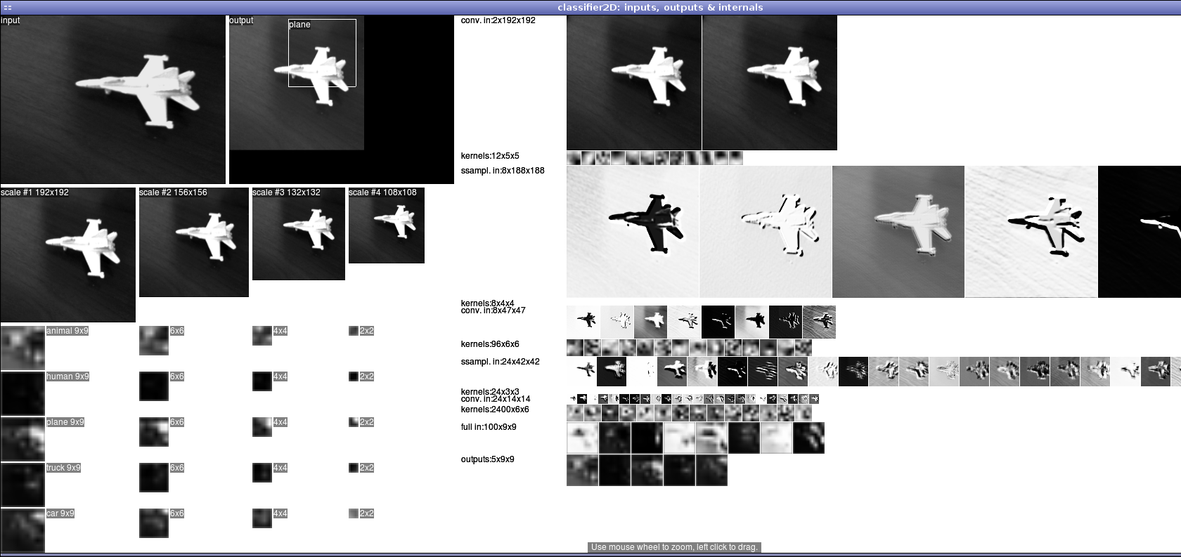
e. Output display of the multi-resolution detection provided by the Classified2D class (top 2 rows, below are the internal network representations). The plane is resized to different resolutions to handle multiple scales and the output of each class for each resolution is shown on the left. The brighter the output, the stronger response for the corresponding class. The 3rd row of the network outputs corresponds to the plane category, which has the strongest responses in the top right of the images, yielding the plane bounding box classification on the right.

Multi-resolution detection: Classifier2D

While the Trainer class takes a module_1_1 and trains it on a dataset, the Classifier2D class takes a trained network as input (loading a 'parameter' saved in an Idx file) to detect objects in images of any size and at different resolution. It resizes the input image to different sizes based on the passed resolutions parameters and applies the network at each scale. Finally, the values in the outputs of the network that are higher than a certain threshold will return a positive detection at the position in the image and a specific scale.

// parameter, network and classifier
// load the previously saved weights of a trained network
parameter theparam(1);
// input to the network will be 96x96 and there are 5 outputs
lenet7_binocular thenet(theparam, 96, 96, 5);
theparam.load_x(mono_net.c_str());
Classifier2D cb(thenet, sz, lbl, 0.0, 0.01, 240, 320);
	  
// find category of image
Idx res = cb.fprop(left.idx_ptr(), 1, 1.8, 60);

Project

Code

Tutorials

Demos

Documentation