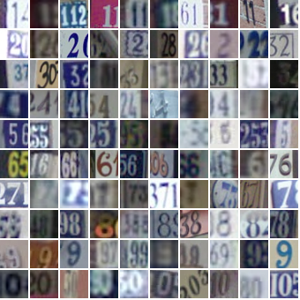
In this tutorial, you will learn how to design, train and test a state-of-the-art classifier for the Stanford/Google Street View House Numbers dataset.

The model is based on Convolutional Networks (ConvNets) which learn all features from scratch rather than using hand-designed features.

More details can be found in the ICPR'12 and Arxiv papers.

1. Install eblearn and go to the svhn demo directory:

   cd eblearn/tools/ && make && make install && make test
   cd eblearn/demos/svhn

   Note: If you cannot install eblearn to the default dir, either install eblearn to another dir and add it to $PATH, or replace calls to each eblearn binary with <eblearn-dir>/bin/<binary-name>

2. Prepare data or download pre-processed data directly (5.6GB):

   wget http://cs.nyu.edu/~sermanet/svhn/svhn_preprocessed.tgz
   tar xzvf svhn_preprocessed.tgz

3. Design and train your model or train an existing model (svhn.conf) by calling:

   train svhn.conf

4. Test your best trained model or test this already trained network (94.85% correct) directly by calling:

   wget http://cs.nyu.edu/~sermanet/svhn/svhn_l4_820.mat
   train svhn_trained.conf

This section explains in more details how to extract and pre-process data, design, train and test a model. You will need approximately 20Gb of disk space for this tutorial. This assumes EBLearn has already been installed and tested. All subsequent commands are assumed to be called from eblearn's demos/svhn folder:

cd eblearn/demos/svhn

1. Download the cropped digits MATLAB matrices from the SVNH website by calling:

   wget http://ufldl.stanford.edu/housenumbers/train_32x32.mat 
   wget http://ufldl.stanford.edu/housenumbers/extra_32x32.mat 
   wget http://ufldl.stanford.edu/housenumbers/test_32x32.mat

2. Use the given matlab script to convert the digits from matlab into images and dump them into labeled folders using

   matlab -nodesktop -nosplash -r svhn_convert_to_images

3. Now use the given python script svhn_dsprepare.py to compile your preprocessed SVHN dataset. We apply a global and locally normalized YUV transform. Note: If your eblearn binaries are not in your system $PATH, look at line 21 of the scripts for instructions.

   python svhn_dsprepare.py

• The model is entirely defined by the svhn.conf configuration file.
• Its architecture is determined by the “arch” variable. To see this architecture, you can either infer it from the configuration file by following its sub-variables definitions or look at the values printed when calling 'train svhn.conf'. Here, “arch” is defined as:

  arch = conv051,addc0,tanh,l4pool22,snorm5,ms2,merge2,linear6,addc6,tanh,linear7,addc7,tanh

• Each module name is composed of the module type followed by an identifier (for example, conv051 is convolution module “conv” with id “051”). The parameters of each module are defined further in the configuration file. For example, the first convolution module “conv051” has the following parameters:

  conv051_kernel=5x5
  conv051_shared=${shared}
  conv051_stride=1x1
  conv051_table=${table0}
  conv051_table_in=1
  conv051_table_out=${table0_max}
  conv051_weights=none.mat

  These parameters indicate that this module performs a 5×5 convolution with stride 1×1, that the features table is found in “table0”, that if “table0” is empty, then it fully connects “table_in” input features to “table_out” outputs features. If “shared” is equal to 1, then all instances of modules which name is “conv051” will share the same weights. Finally, if “none.mat” exists and “manual_load” is set to 1, the internal weights will be initialized with these rather than randomly.

• You can easily experiment with different model parameters and modules, for example using an L2 pooling instead of L4, or use a 1-layer linear classifier (linear6,addc6,tanh) instead of a 2-layer non-linear classifier (linear6,addc6,tanh,linear7,addc7,tanh).
• Other hyper-parameters can also be tuned, such as learning rate “eta” or regularization “reg”.

• Run the training

  train svhn.conf

• This model typically takes around 10 minutes per iteration (where an iteration see 10,000 training samples and 6,000 validation samples).
• The training and validation error is displayed after each iteration (uerrors and ucorrect, errors and correct are the class-normalized rates, i.e. taking into account the number of samples for each class).
• The training will converge after approximately 800 iterations.
• You can expect a validation error rate of ~7.5% after 100 iterations, ~6.6% after 200 iterations, ~6.2% after 500 iterations and ~5.9% after 1000 iterations.
• The results will slightly vary based on the random training/validation split and the random weights initialization.

1. Select an iteration that obtained the lowest validation error and identify its corresponding weight file. This file's name will look like this: *_net{iteration_number}.mat.
2. Add the following lines at the end of the file “svhn.conf”

   retrain_weights=[weights-filename]
   retrain=1
   test_only = 1
   test_dsname= svhn_ynuv7_test
   val_dsname = ${test_dsname} # for testing, replace val by test 
   training_precision = float # takes advantage of float optimizations

3. Rerun the train binary on the conf

   train svhn.conf

4. At the end of the testing, “test_ucorrect=” indicates the success rate of the model on the testing set.